R for predicting kidney transplant success

Simon Schwab

Swisstransplant, Bern

Center for Reproducible Science and Research Synthesis, University of Zurich

16. September 2026

Kidney transplant

• It is challanging to make clinical predictions
• From development, validation to implementation
• More an art than a science (to be honest)

Study objective

KIDMO is a clinical prediction model to estimate graft loss risk in deceased-donor kidney transplantation. It uses a combination of

• donor and
• recipient clinical characteristics.

Goal

Inform clinicians and patients of individual outcome risks at the time of organ offer to support decision-making and improve outcomes.

Clinical prediction models play a vital role in advancing personalized medicine.

Design, participants, setting and outcome

Design	National multi-center retrospective cohort study.
Participants	All deceased-donor kidney transplant recipients from 2008 to 2021.
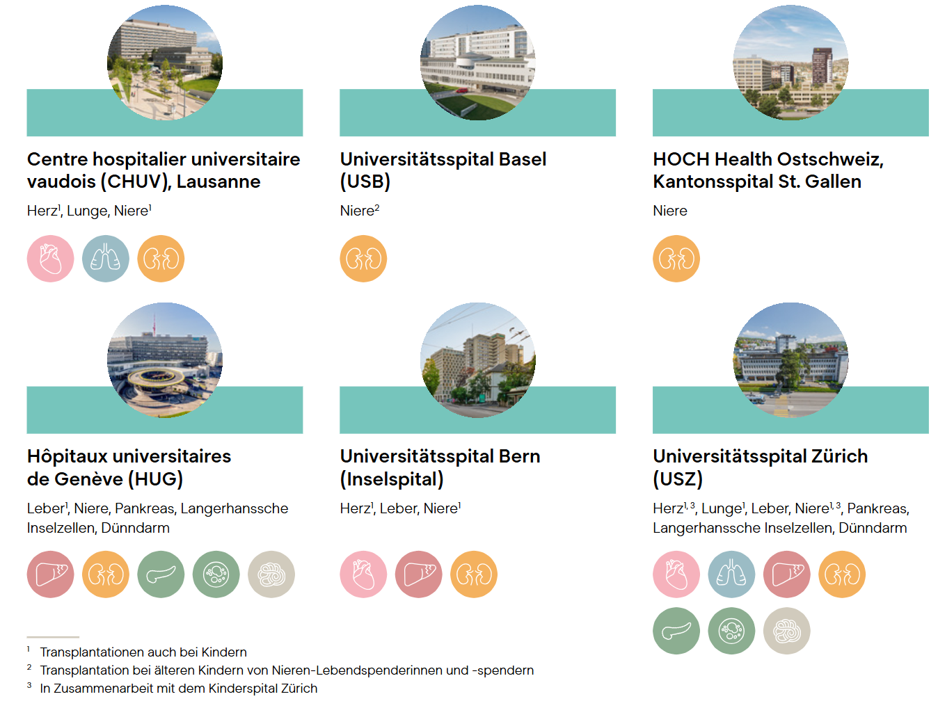
Setting	Six Swiss transplant centers: Basel, Bern, Geneva, Lausanne, St. Gallen, and Zurich.
Primary Outcome	Time to graft loss (interval from transplantation to irreversible graft failure). Patient death was treated as a competing risk.

Swiss transplant centers

Methods

• Competing risk regression (Fine & Gray model)
• Non-linear modelling (restricted cubic splines)
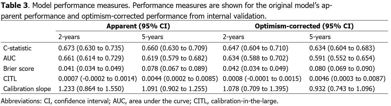
• Model performance: C-statistic, area under the curve (AUC), Brier score, calibration plot, calibration in-the-large, calibration slope
• Internal validation and optimism correction (bootstrapping with B=1,000)
• Internal-external cross-validation
• Clinical utility (decision curve analysis and net benefit)

Study protocol

We published a study protocol.¹

• Prespecified predictors
• Sample size calculation²
• N=2,042 recipients
• 167 events
• 19 parameters (16 variables)
• EPP 8.8
• Statistical analysis plan

1. Schwab et al. 2023, Diagn Progn Res

2. Riley et al. 2020, BMJ

Participant flow

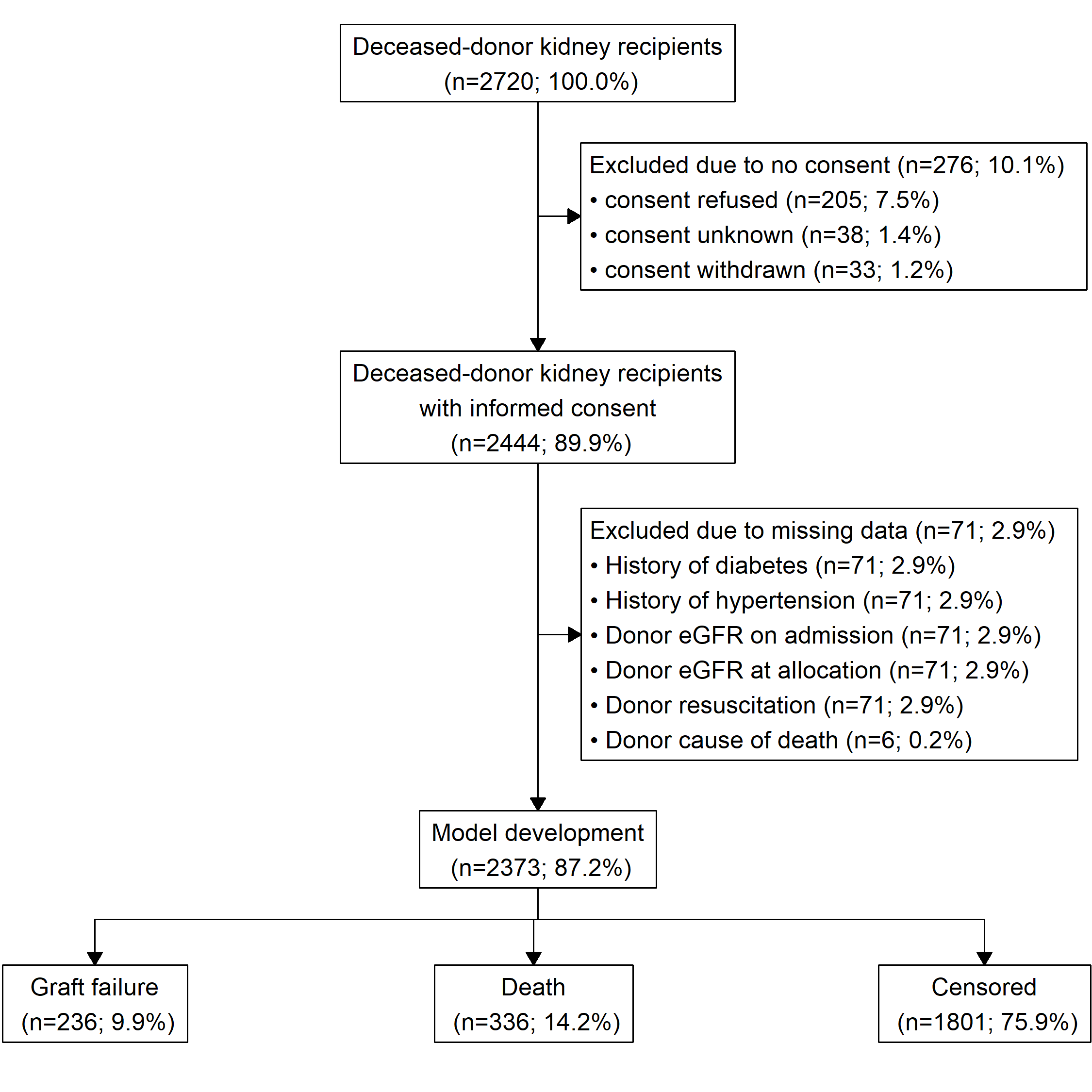
87% of the population in the model development.

Exclusion:

• 10.1% with no consent
• 2.9% missing data

Dropouts (were censored):

• 34 (1.4%) dropouts
• 33 moved away
• 1 other reason

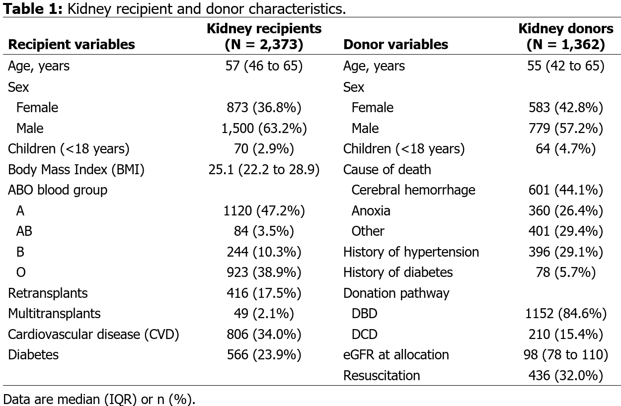
Receipient and donor characteristics

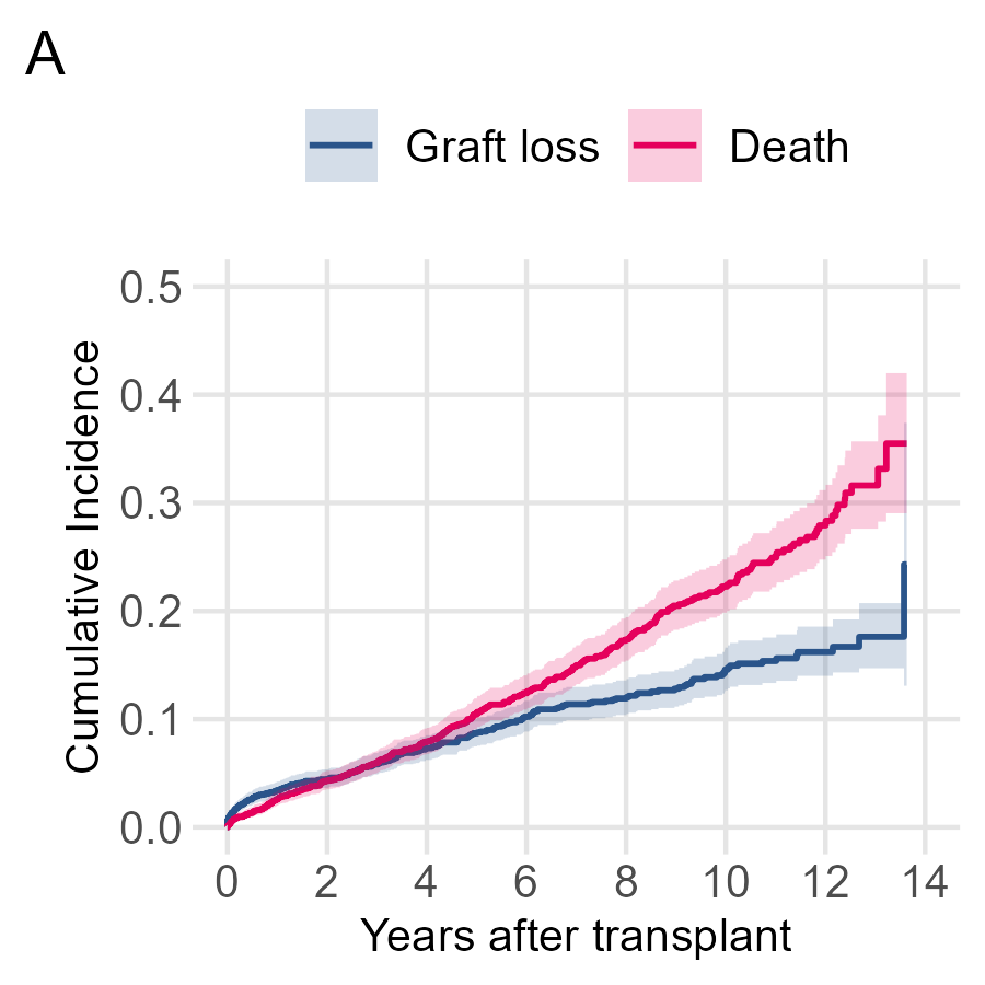
Cumulative incidence

Probability of an event by time t (with 95% confidence bands).

Outcome	2-years	5-y years
Graft loss	4.4% (3.6–5.3)	8.7% (7.4–10.0)
Death	4.3% (3.5–5.2)	10.4% (9.0–11.9)

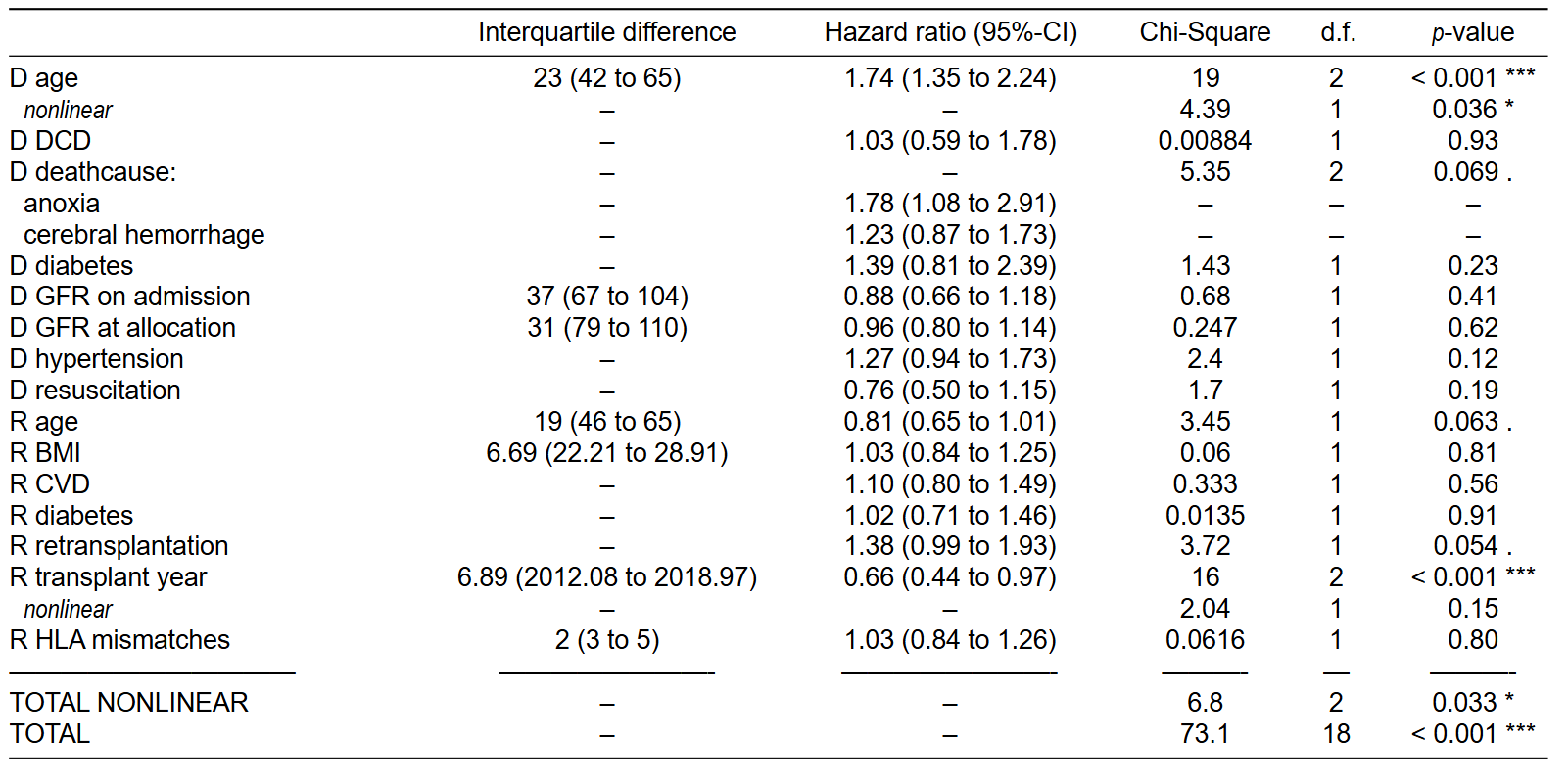
Full model

• 15 predictor variables altogether
  • not included: recipient DSA, recipient time on dialysis (missing data)
  • additionally included: transplant year

Variable selection

• Backward elimination with AIC (p≈0.157) across 1,000 bootstraps¹
• Selection criterion: variables contained in at least 50% of the time

→ Entire model-building process was repeated within each bootstrap

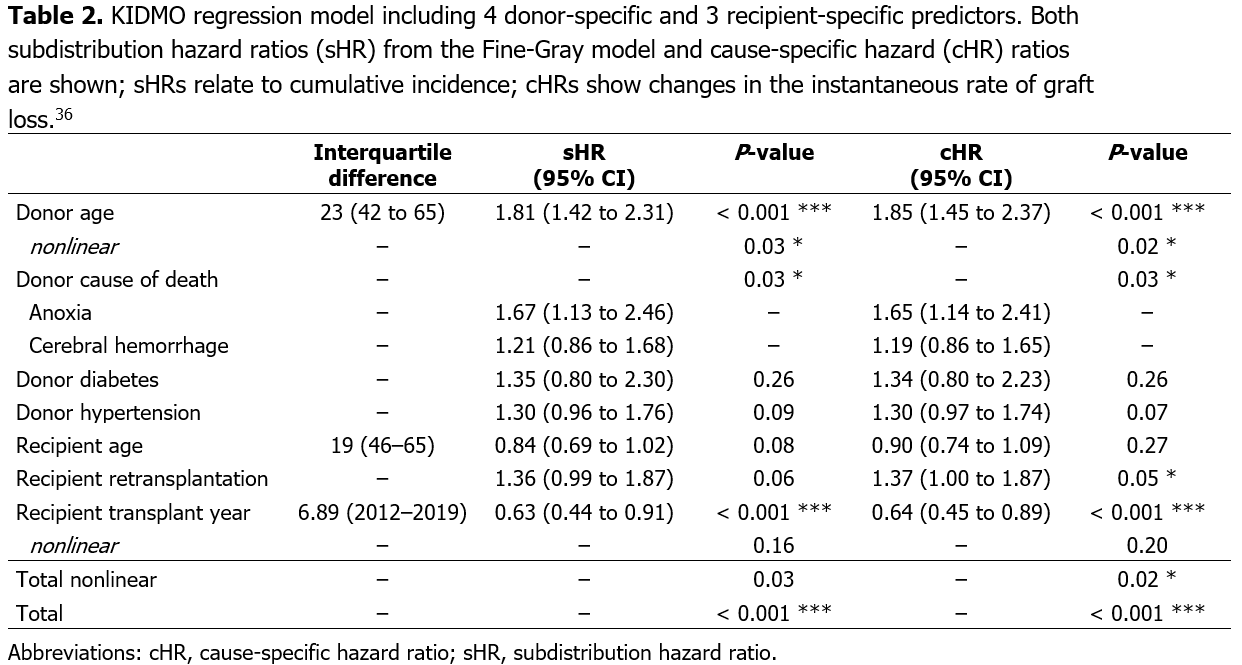
Final model

• 7 variables
  • 4 donor variables
  • 3 recipient variables

1. Heinze & Dunkler, 2017, Transpl Int

Final model

Not all predictors are statistically significant and that is okey.

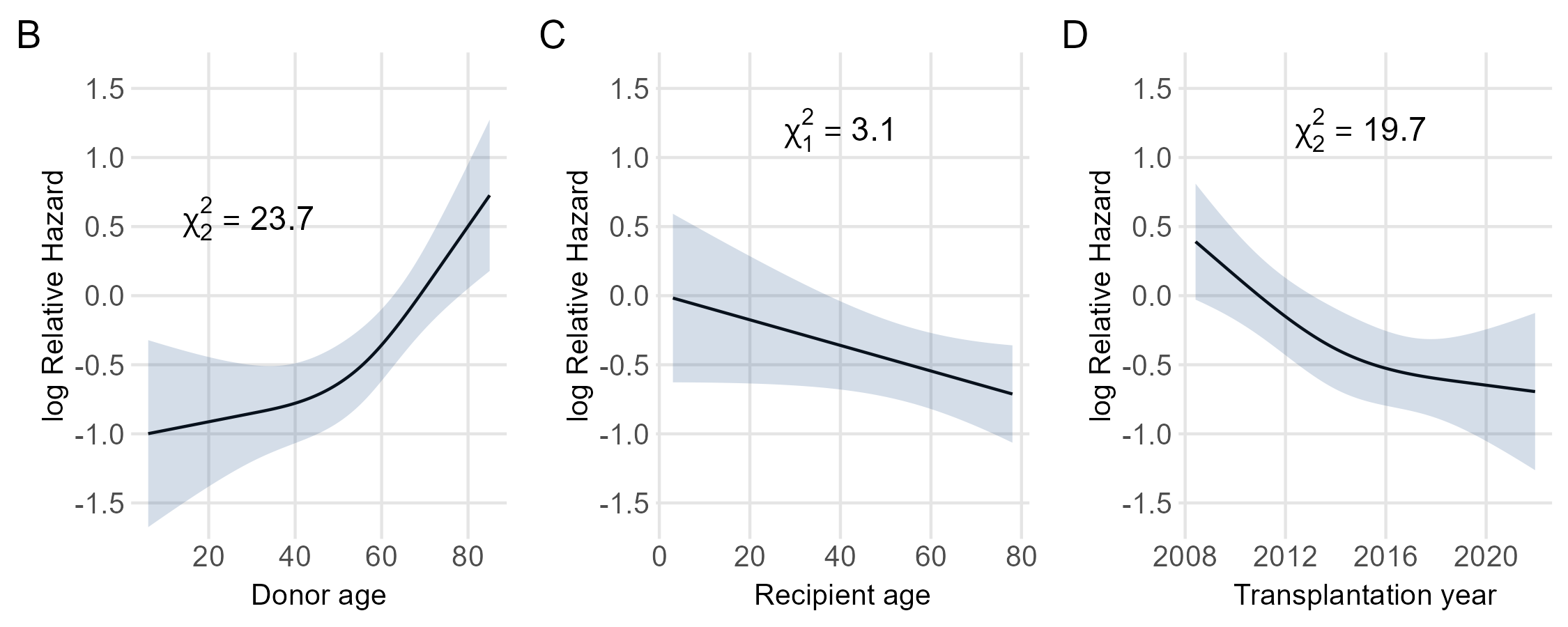
Partial effects

Partial effects of the continuous variables (B) donor age, (C) recipient age, and (D) transplantation year on the graft loss rate.

• Reveals important relationship with outcome
• Does it make sense, clinically?

Performance measures

• Modest discrimination
• Good calibration

Model equation

Uer the Fine–Gray formulation, the subdistribution hazard leads to the following expression for the graft-survival function:

\[\Pr(T\geq t~|~X) = S_{0}(t)^{\mathrm{e}^{X\beta}},\]

where \(S_{0}(t)\) denotes the baseline survival function. Baseline survival values used for prediction are provided in the table below for the clinically relevant time points \(t = 2\) and \(t = 5\) years.

\(t\)	\(S_{0}(t)\)
2	0.9594
5	0.9225

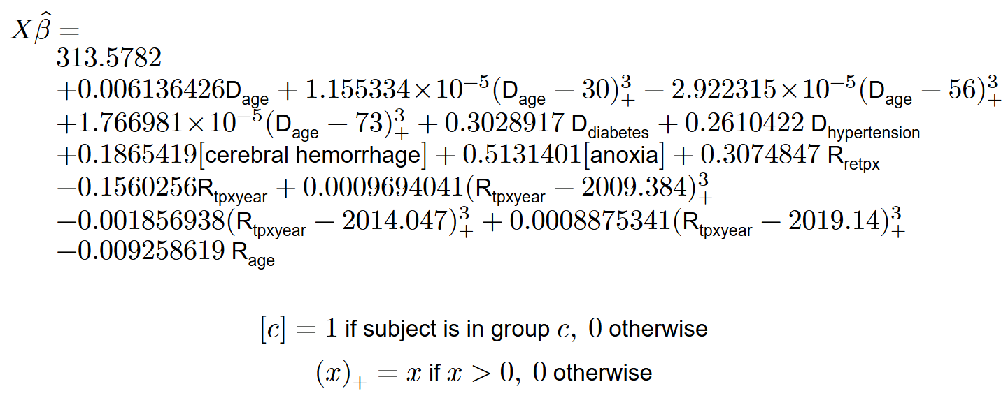
Linear predictor

The term \(\mathrm{e}^{X\beta}\) is the individual-specific subdistribution hazard ratio derived from the linear predictor \(X\hat{\beta}\) shown below.

Absolute risks

The cumulative incidence, i.e., the probability of graft loss by time \(t\) for an individual with covariates \(X\), is

\[ F(t~|~X) = 1 - S_{0}(t)^{\textrm{e}^{X\beta}}, \]

where

• \(S_0(t)\) is the baseline graft survival function at time \(t\), and
• \(\textrm{e}^{X\beta}\) is the hazard ratio, obtained from the linear predictor.

Accordingly, the cumulative incidence at 2 and 5 years after transplant is given by:

• 2-year risk: \(F(t = 2 | X) = 1 - S_{0}(2)^{\textrm{e}^{X\beta}}\) = \(1 - \textrm{0.959}^{\textrm{e}^{X\beta}}\),
• 5-year risk: \(F(t = 5 | X) = 1 - S_{0}(5)^{\textrm{e}^{X\beta}}\) = \(1 - \textrm{0.922}^{\textrm{e}^{X\beta}}\).

Implementation in Swisstransplant package swt

The KIDMO risk score has been implemented in the Swisstransplant R package swt.

• https://data.swisstransplant.org/tools/
• enable easy calculation of the KIDMO score (among other stuff)

remotes::install_github("Swisstransplant/swt")

kidmo() function

Usage

library(swt)

kidmo(D_age = 45,
      D_deathcause = "anoxia",
      D_diabetes = TRUE,
      D_hypertension = TRUE,
      R_age = 50,
      R_retpx = TRUE,
      R_tpxyear = 2026)

KIDMO Risk Score
Number of recipients: 1 
Summary:
  kidmo rank 2-year risk 5-year risk
1  1.46  75%  0.05279943   0.1003058

• Easy calculation of example patient

Option newdata

data = data.frame(D_age = 45,
                  D_deathcause = "anoxia",
                  D_diabetes = TRUE,
                  D_hypertension = TRUE,
                  R_age = 50,
                  R_retpx = TRUE,
                  R_tpxyear = 2026)

stats = kidmo(newdata = data)
stats

KIDMO Risk Score
Number of recipients: 1 
Summary:
  kidmo rank 2-year risk 5-year risk
1  1.46  75%  0.05279943   0.1003058

• Practical when dealing with large data

Behind the scenes

• Model fit is stored as internal data in sysdata.rda (cph object from rms)

# Quality checks: don't save sensitive data
idat.kidmo.model$x = NULL
assert(is.null(idat.kidmo.model$x))

usethis::use_data(
  idat.kidmo.model,
  internal = TRUE, overwrite = TRUE
)

• Write function to access internal data
  • use predict() to get linear predictor
  • calculate relative and absolute risks (textbook formulas)

Careful, do not leak any patient level data!

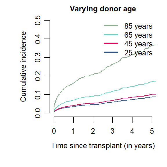
An example with donor age

Let’s create 4 kidney recipients with varying donor age, other factors being equal:

data = data[rep(1,4), ]
data$D_age = c(25, 45, 65, 85)

stats = kidmo(newdata = data)
stats$summary

kidmo	rank	2-year risk	5-year risk
1.25	65%	0.0450961	0.0859930
1.46	75%	0.0527994	0.1003058
2.56	94%	0.0904031	0.1685937
6.22	100%	0.2058106	0.3617473

Plots

The returned object also includes the cumulative incidence curves, see stats$CI and stats$CI.time (stats$CI.lower and stats$CI.upper for 95% CI).

Cumulative incidence curves for recipients of kidneys from donors of varying ages, all other factors being equal.

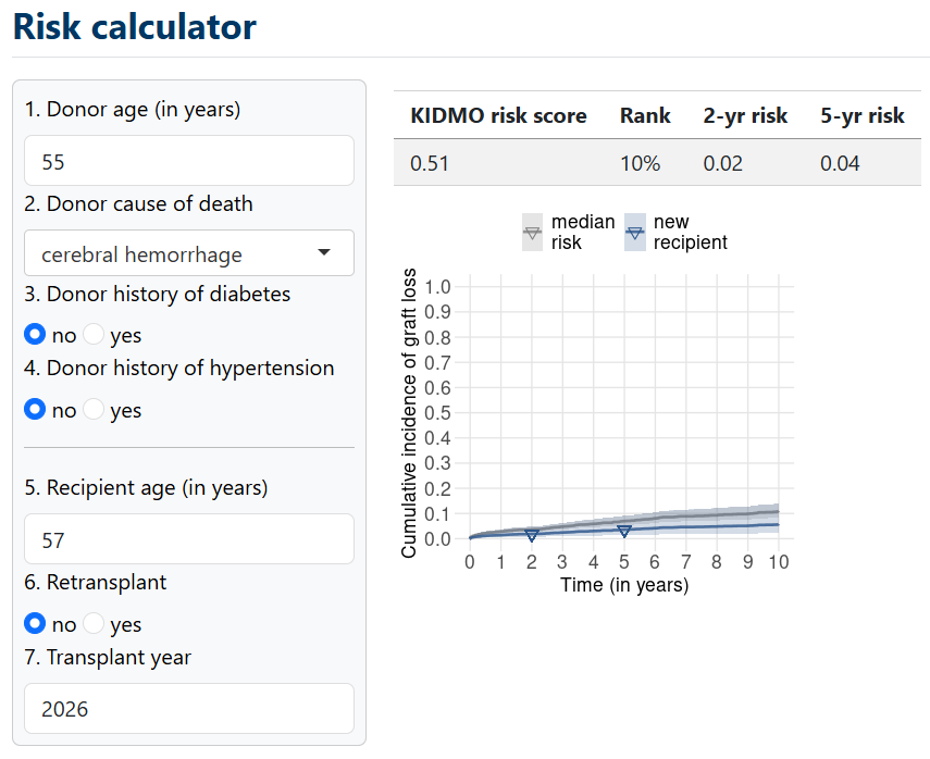
Online risk calculator

• Shiny app runs on Posit Connect Cloud
• Quarto website implements app with HTML iframe
• https://data.swisstransplant.org/kidmo/

Code in Quarto Website:

<iframe id="KIDMO" src="https://swisstransplant-kidmo-app.share.connect.posit.cloud" style="border: none; width: 100%; height: 570px" frameborder="0"></iframe>

Awesome tools

• R and RStudio
• Quarto Documents / Websites / Presentations / Dashboards
• Posit Connect Cloud
• GitHub / GitHub pages